UNIT-II
Image enhancement : point operations – contrast stretching, clipping and thresholding – Histogram modeling – Spatial operations – averaging and low pass filtering, smoothing filter, sharpening filter and median filtering - Image Enhancement in frequency domain – smoothing and sharpening filters – Homomorphic filter
Point Operations
Contents
 Thresholding - select pixels with given values to produce binary image
 Adaptive Thresholding - like Thresholding except choose values locally
 Contrast Stretching - spreading out graylevel distribution
 Histogram Equalization - general method of modifying intensity distribution
 Logarithm Operator - reducing contrast of brighter regions
 Exponential/`Raise to Power' Operator - enhancing contrast of brighter regions
Single-point processing is a simple method of  image enhancement. This technique determines a pixel value in the enhanced image dependent only on the value of the corresponding pixel in the input image. The process can be described with the
  mapping function
where r and s are the pixel values in the input and output images, respectively. The form of the mapping function M determines the effect of the operation. It can be previously defined in an ad-hoc manner, as for thresholding or gamma correction, or it can be computed from the input image, as for histogram equalization. For example, a simple mapping function is defined by the thresholding operator:
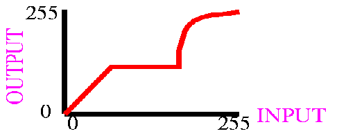
The corresponding graph is shown in Figure 1.
Figure 1 Graylevel transformation function for thresholding.
Point operators are also known as  LUT-transformations, because the mapping function, in the case of a discrete image, can be implemented in a look-up table (LUT).
A subgroup of the point processors is the set of  anamorphosis operators. This notion describes all point operators with a strictly increasing or decreasing mapping function. Examples include the logarithm operator, exponential operator and contrast stretching, to name just a few.
An operator where M changes over the image is adaptive thresholding. This is not a pure point operation anymore, because the mapping function, and therefore the output pixel value, depends on the local neighborhood of a pixel.
Contrast stretching, clipping and thresholding:-Contrast stretching (often called normalization) is a simple image enhancement technique that attempts to improve the contrast in an image by 'stretching' the range of intensity values it contains to span a desired range of values, the full range of pixel values that the image type concerned allows.
Contrast Stretching
Common Names: Contrast stretching, Normalization
Brief Description
Contrast stretching (often called normalization) is a simple image enhancement technique that attempts to improve the contrast in an image by `stretching' the range of intensity values it contains to span a desired range of values, e.g. the the full range of pixel values that the image type concerned allows. It differs from the more sophisticated histogram equalization in that it can only apply a linear scaling function to the image pixel values. As a result the `enhancement' is less harsh. (Most implementations accept a graylevel image as input and produce another graylevel image as output.)
How It Works
Before the stretching can be performed it is necessary to specify the upper and lower pixel value limits over which the image is to be normalized. Often these limits will just be the minimum and maximum pixel values that the image type concerned allows. For example for 8-bit graylevel images the lower and upper limits might be 0 and 255. Call the lower and the upper limits a and b respectively.
The simplest sort of normalization then scans the image to find the lowest and highest pixel values currently present in the image. Call these c and d. Then each pixel P is scaled using the following function:
Values below 0 are set to 0 and values about 255 are set to 255.
The problem with this is that a single outlying pixel with either a very high or very low value can severely affect the value of c or d and this could lead to very unrepresentative scaling. Therefore a more robust approach is to first take a histogram of the image, and then select c and d at, say, the 5th and 95th percentile in the histogram (that is, 5% of the pixel in the histogram will have values lower than c, and 5% of the pixels will have values higher than d). This prevents outliers affecting the scaling so much.
Another common technique for dealing with outliers is to use the intensity histogram to find the most popular intensity level in an image (i.e. the histogram peak) and then define a cutoff fraction which is the minimum fraction of this peak magnitude below which data will be ignored. The intensity histogram is then scanned upward from 0 until the first intensity value with contents above the cutoff fraction. This defines c. Similarly, the intensity histogram is then scanned downward from 255 until the first intensity value with contents above the cutoff fraction. This defines d.
Some implementations also work with color images. In this case all the channels will be stretched using the same offset and scaling in order to preserve the correct color ratios.
Guidelines for Use
Normalization is commonly used to improve the contrast in an image without distorting relative graylevel intensities too significantly.
We begin by considering an image
which can easily be enhanced by the most simple of contrast stretching implementations because the intensity histogram forms a tight, narrow cluster between the graylevel intensity values of 79 - 136, as shown in
After contrast stretching, using a simple linear interpolation between c = 79 and d = 136, we obtain
Compare the histogram of the original image with that of the contrast-stretched version
While this result is a significant improvement over the original, the enhanced image itself still appears somewhat flat. Histogram equalizing the image increases contrast dramatically, but yields an artificial-looking result
In this case, we can achieve better results by contrast stretching the image over a more narrow range of graylevel values from the original image. For example, by setting the cutoff fraction parameter to 0.03, we obtain the contrast-stretched image
and its corresponding histogram
Note that this operation has effectively spread out the information contained in the original histogram peak (thus improving contrast in the interesting face regions) by pushing those intensity levels to the left of the peak down the histogram x-axis towards 0. Setting the cutoff fraction to a higher value, e.g. 0.125, yields the contrast stretched image
As shown in the histogram
most of the information to the left of the peak in the original image is mapped to 0 so that the peak can spread out even further and begin pushing values to its right up to 255.
As an example of an image which is more difficult to enhance, consider
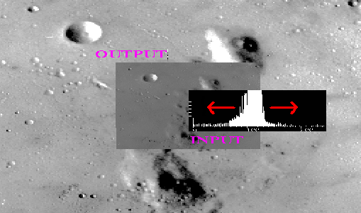
which shows a low contrast image of a lunar surface.
The image
shows the intensity histogram of this image. Note that only part of the y-axis has been shown for clarity. The minimum and maximum values in this 8-bit image are 0 and 255 respectively, and so straightforward normalization to the range 0 - 255 produces absolutely no effect. However, we can enhance the picture by ignoring all pixel values outside the 1% and 99% percentiles, and only applying contrast stretching to those pixels in between. The outliers are simply forced to either 0 or 255 depending upon which side of the range they lie on.
shows the result of this enhancement. Notice that the contrast has been significantly improved. Compare this with the corresponding enhancement achieved using histogram equalization.
Normalization can also be used when converting from one image type to another, for instance from floating point pixel values to 8-bit integer pixel values. As an example the pixel values in the floating point image might run from 0 to 5000. Normalizing this range to 0-255 allows easy conversion to 8-bit integers. Obviously some information might be lost in the compression process, but the relative intensities of the pixels will be preserved.
Interactive Experimentation
You can interactively experiment with this operator by clicking here.
Exercises
- Derive the scaling formula given above from the parameters a, b, c and d.
- Suppose you had to normalize an 8-bit image to one in which the pixel values were stored as 4-bit integers. What would be a suitable destination range (i.e. the values of a and b)?
- Contrast-stretch the image
(You must begin by selecting suitable values for c and d.) Next, edge-detect (i.e. using the Sobel, Roberts Cross or Canny edge detector) both the original and the contrast stretched version. Does contrast stretching increase the number of edges which can be detected?
There are 3 customers waiting between 1 and 35 seconds. There are 5 customers waiting between 1 and 40 seconds. There are 5 customers waiting between 1 and 45 seconds. There are 5 customers waiting between 1 and 50 seconds.
7.3.7 Buffer zones
One other class of spatial operations includes the creation of boundaries, inside or outside an existing polygon, offset by a certain distance, and parallel to the boundary. Referred to, respectively, by the terms skeleton and buffer zones, these new units require distance measures from selected points on the boundary of the polygon (Figure 7.16a). The skeleton is akin to contracting the polygon by moving straight line segments in, parallel to their original position, and the buffer has lines moving outwards. Skeletons (Figure 7.16b) have some value in assisting labelling operations for polygons or edges; buffers are much used in spatial analysis and modelling.
Figure 7.16. The concepts of buffers. (a) Buffer zones. (b) Skeleton zones. (c) Example of a buffer zone for major roads.
For example, as demonstrated in Figure 2.18, buffers are used to establish critical areas for analysis or to indicate proximity or accessibility conditions. In contrast to the simpler world of proximity values for grid cell data, for vector data, computational geometry operations are required to establish buffer zones. If the concept of gradation in accessibility is required, then a sequence of buffers at selected increasing distances must be created. Similarly, for a zone within two specified distances, two new buffer boundaries have to be determined (Figure 7.16c). If a vector data representation is required, then this buffering operation is best done as a batch or background process because of the time it can take. In contrast, the equivalent operation for regular tessellations can be done much faster because it does not need to employ time consuming computational geometry operations.
Full Detail Pdf:- Click Hear Pdf
Averaging and low pass filtering:-
A low pass filter is the basis for most smoothing methods. An image is smoothed by decreasing the disparity between pixel values by averaging nearby pixels. Using a low pass filter tends to retain the low frequency information within an image while reducing the high frequency information.
Homomorphic filtering – part 1
Posted by Steve Eddins,
I'd like to welcome back guest blogger Spandan Tiwari for today's post. Spandan, a developer on the Image Processing Toolbox team, posted here previously about circle finding.
Recently I attended a friend's wedding at an interesting wedding venue, the Charles River Museum of Industry and Innovation in the town of Waltham, not very far from the Mathworks headquarters here in Natick. While waiting for the guests to arrive, we all got a chance to look around the museum. It's a nice little place with several quirky old machines on display, some dating back to 1812. Hanging on a wall in a dimly lit corner of the museum was a framed copy of an engineer's decadic logarithm (and anti-logarithm) tables. A friend who was looking around with me commented, "Ah, logs...haven't seen these since school days." That got me thinking. When was the last time I used logarithms? Well, just in the morning I had used the log function for scaling the Fourier magnitude spectrum of an image for better visualization. It took me a moment though to make the mental connection between the printed log tables and log's functional form, but as soon as I did, I realized that I used log quite often.
It also reminded me of a neat image enhancement technique from the olden days of image processing called homomorphic filtering, which makes clever use of the log function. There are several image denoising/enhancement techniques in literature that assume an additive noise model, i.e.
Homomorphic filtering is one such technique for removing multiplicative noise that has certain characteristics.
Homomorphic filtering is most commonly used for correcting non-uniform illumination in images. The illumination-reflectance model of image formation says that the intensity at any pixel, which is the amount of light reflected by a point on the object, is the product of the illumination of the scene and the reflectance of the object(s) in the scene, i.e.,
where
Illumination typically varies slowly across the image as compared to reflectance which can change quite abruptly at object edges. This difference is the key to separating out the illumination component from the reflectance component. In homomorphic filtering we first transform the multiplicative components to additive components by moving to the log domain.
Then we use a high-pass filter in the log domain to remove the low-frequency illumination component while preserving the high-frequency reflectance component. The basic steps in homomorphic filtering are shown in the diagram below:

For a working example I will use an image from the Image Processing Toolbox.
I = imread('AT3_1m4_01.tif');
imshow(I)
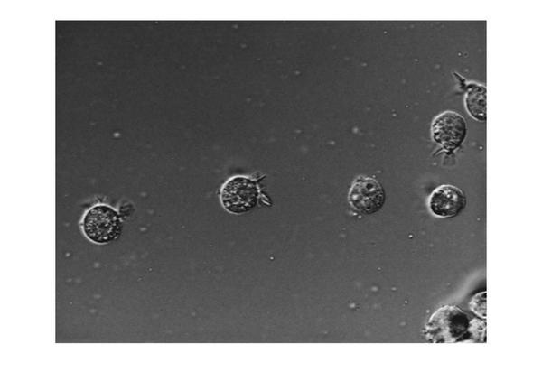
In this image the background illumination changes gradually from the top-left corner to the bottom-right corner of the image. Let's use homomorphic filtering to correct this non-uniform illumination.
The first step is to convert the input image to the log domain. Before that we will also convert the image to floating-point type.
I = im2double(I);
I = log(1 + I);
The next step is to do high-pass filtering. We can do high-pass filtering in either the spatial or the spectral domain. Although they are both exactly equivalent, each domain offers some practical advantages of its own. We will do both it ways. Let's start with frequency-domain filtering. In frequency domain the homomorphic filtering process looks like:

First we will construct a frequency-domain high-pass filter. There are different types of high-pass filters you can construct, such as Gaussian, Butterworth, and Chebychev filters. We will construct a simple Gaussian high-pass filter directly in the frequency domain. In frequency domain filtering we have to careful about the wraparound error which comes from the fact that Discrete Fourier Transform treats a finite-length signal (such as the image) as an infinite-length periodic signal where the original finite-length signal represents one period of the signal. Therefore, there is interference from the non-zero parts of the adjacent copies of the signal. To avoid this, we will pad the image with zeros. Consequently, the size of the filter will also increase to match the size of the image.
M = 2*size(I,1) + 1;
N = 2*size(I,2) + 1;
Note that we can make the size of the filter (M,N) even numbers to speed-up the FFT computation, but we will skip that step for the sake of simplicity. Next, we choose a standard deviation for the Gaussian which determines the bandwidth of low-frequency band that will be filtered out.
sigma = 10;
And create the high-pass filter...
[X, Y] = meshgrid(1:N,1:M);
centerX = ceil(N/2);
centerY = ceil(M/2);
gaussianNumerator = (X - centerX).^2 + (Y - centerY).^2;
H = exp(-gaussianNumerator./(2*sigma.^2));
H = 1 - H;
Couple of things to note here. First, we formulate a low-pass filter and then subtracted it from 1 to get the high-pass filter. Second, this is a centered filter in that the zero-frequency is at the center.
imshow(H,'InitialMagnification',25)
We can rearrange the filter in the uncentered format using fftshift.
H = fftshift(H);
Next, we high-pass filter the log-transformed image in the frequency domain. First we compute the FFT of the log-transformed image with zero-padding using the fft2 syntax that allows us to simply pass in size of the padded image. Then we apply the high-pass filter and compute the inverse-FFT. Finally, we crop the image back to the original unpadded size.
If = fft2(I, M, N);
Iout = real(ifft2(H.*If));
Iout = Iout(1:size(I,1),1:size(I,2));
The last step is to apply the exponential function to invert the log-transform and get the homomorphic filtered image.
Ihmf = exp(Iout) - 1;
Let's look at the original and the homomorphic-filtered images together. The original image is on the left and the filtered image is on the right. If you compare the two images you can see that the gradual change in illumination in the left image has been corrected to a large extent in the image on the right.
imshowpair(I, Ihmf, 'montage')
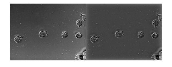
Next time we will explore homomorphic filtering some more. We will see a slightly modified form of homomorphic filtering and also discuss why we might want to do filtering in the spatial domain.


