UNIT-I

Introduction : Image perception – light, luminance, brightness and contrast – Monochrome vision models – Image fidelity criteria – color representation. Digital image sampling and quantization –Basic relationship between pixels

Introduction : Image perception:-

Mirror-image perception is the human tendency to see oneself (especially while in the throes of conflict) as the opposite of the person with whom they are having a conflict. They are mutual and reciprocal views of others.

Detail:- Click hear Pdf

Light, luminance, brightness and contrast:-

Contrast is to black level as brightness is to luminance. Generally, contrast control is performed by adjusting the black level, or the amount of light emitted or transmitted by the low end of the display output. Note that these controls work differently on other display types, such as CRTs.

What is the difference between lightness and luminance?

Luminance on the other hand is a measure to describe the perceived brightness of a color (Encyclopædia Britannica: "luminance, or visually perceived brightness"). You can lighten or darken a color by adjusting its lightness value, but lightness is not the only dimension to consider for luminance.

What is the difference between contrast and brightness?

Contrast is to black level as brightness is to luminance. Generally, contrast control is performed by adjusting the black level, or the amount of light emitted or transmitted by the low end of the display output.

Monochrome Vision Model

Last Updated on Tue, 27 Dec 2021 | Image Processing

One of the modern techniques of optical system design entails the treatment of an optical system as a two-dimensional linear system that is linear in intensity and can be characterized by a two-dimensional transfer function (17). Consider the linear optical system of Figure 2.4-1. The system input is a spatial light distribution obtained by passing a constant-intensity light beam through a transparency with a spatial sine-wave transmittance. Because the system is linear, the spatial output intensity distribution will also exhibit sine-wave intensity variations with possible changes in the amplitude and phase of the output intensity compared to the input intensity. By varying the spatial frequency (number of intensity cycles per linear dimension) of the input transparency, and recording the output intensity level and phase, it is possible, in principle, to obtain the optical transfer function (OTF) of the optical system.

Let rny) represent the optical transfer function of a two-dimensional linear system where rnx = 2n/Tx and rny = 2n/Ty are angular spatial frequencies with spatial periods Tx and Ty in the x and y coordinate directions, respectively. Then, with ¡¡(x, y) denoting the input intensity distribution of the object and Io(x, y)

: FIGURE 2.4-1. Linear systems analysis of an optical system.

representing the output intensity distribution of the image, the frequency spectra of the input and output signals are defined as

I(<x> <y) = J"°° J°° x y)exp{-i(axx + <yy)} dxdy (2.4-1)

Io(<x-<y) = J1J1 Jo(x, y)exp{-i(raxx + <yy)} dxdy (2.4-2)

The input and output intensity spectra are related by

Io(<x, <y) = H(<x, <y)I(<x, <y) (2.4-3)

The spatial distribution of the image intensity can be obtained by an inverse Fourier transformation of Eq. 2.4-2, yielding

Jo(x, y) = ¡Z,jZ,Io(<x' <y) exp {i(<xx + <yy)} d<xd<y (2.4-4)

In many systems, the designer is interested only in the magnitude variations of the output intensity with respect to the magnitude variations of the input intensity, not the phase variations. The ratio of the magnitudes of the Fourier transforms of the input and output signals, is called the modulation transfer function (MTF) of the optical system.

Much effort has been given to application of the linear systems concept to the human visual system (18-24). A typical experiment to test the validity of the linear systems model is as follows. An observer is shown two sine-wave grating transparencies, a reference grating of constant contrast and spatial frequency and a variable-contrast test grating whose spatial frequency is set at a value different from that of the reference. Contrast is defined as the ratio max---min max + min where max and min are the maximum and minimum of the grating intensity, respectively. The contrast of the test grating is varied until the brightnesses of the bright and dark regions of the two transparencies appear identical. In this manner, it is possible to develop a plot of the MTF of the human visual system. Figure 2.4-2a is ahypothetical plot of the MTF as a function of the input signal contrast. Another indication of the form of the MTF can be obtained by observation of the composite sine-wave grating of Figure 2.4-3, in which spatial frequency increases in one

: FIGURE 2.4-2. Hypothetical measurements of the spatial frequency response of the human visual system.

FIGURE 2.4-3. MTF measurements of the human visual system by modulated sine-wave grating.

Fidelity criteria

When lossy compression techniques are employed, the decompressed image will not be identical to the original image. In such cases , we can define fidelity criteria that measure the difference between this two images. Two general classes of criteria are used:(1) objective fidelity criteria and (2)subjective fidelity criteria. Subjective: based on human observers. Objective: mathematically defined criteria.

Detail:- Click Hear Pdf

Color representation. Digital image sampling and quantization :-

6 Difference Between Sampling And Quantization In Digital Image Processing

An image function f(x,y) must be digitized both spatially and in amplitude in order to become suitable for digital processing. Typically, a frame grabber or digitizer is used to sample and quantize the analogue video signal. Therefore, in order to create an image which is digital, we need to convert continuous data into digital form. This conversion from analog to digital involves two processes:

Sampling (digitization of coordinate values).
Quantization (digitization of amplitude values).

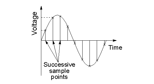
Sampling

In digital image processing, sampling is the reduction of a continuous-time signal to a discrete-time signal. Sampling can be done for functions varying in space, time or any other dimension and similar results are obtained in two or more dimensions. Sampling takes two forms: Spatial and temporal. Spatial sampling is essentially the choice of 2D resolution of an image whereas temporal sampling is the adjustment of the exposure time of the CCD. Sampling is done on x-axis whereby infinite values are converted to digital values.

What You Need To Know About Sampling

Sampling is the reduction of a continuous-time signal to a discrete-time signal.
In sampling, the values on the y-axis, usually amplitude, are continuous but the time or x-axis is discretized.
Sampling is done prior to the quantization process.
The sampling rate determines the spatial resolution of the digitized image.
Sampling reduces a continuous curve (Time-Amplitude Graph) to a series of “tent poles” over time.
In the sampling process, a single amplitude value is selected from different values of the time interval to represent it.

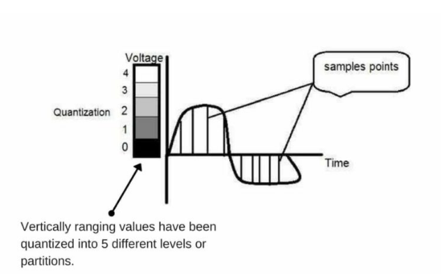
Quantization

Quantization is the process of mapping input values from a large set to output values in a smaller set, often with a finite number of elements. Quantization is the opposite of sampling. It is done on the y-axis. When you are quantizing an image, you are actually dividing a signal into quanta (partitions). On the x axis of the signal, are the coordinate values and on the y-axis, we have amplitudes. Therefore, digitizing the amplitudes is what is referred to as quantization.

What You Need To Know About Quantization

The transition between continuous values of the image function and its digital equivalent is referred to as quantization.
Quantization makes a sampled signal truly digital and ready for processing by a computer.
In quantization, time or x-axis is continuous and the y-axis or amplitude is discretized.
Quantization is done after sampling process.
The quantization level determines the number of grey levels in the digitized image.
Quantization reduces a continuous curve to a continuous series of ‘’stair steps’’ that exist at regular time interval.
In quantization process, the values representing the time intervals are rounded off, to create a defined set of possible amplitude values.

Difference Between Sampling And Quantization In Tabular Form

BASIS OF COMPARISON	SAMPLING	QUANTIZATION
X And Y axis	In sampling, the values on the y-axis, usually amplitude, are continuous but the time or x-axis is discretized.	In quantization, time or x-axis is continuous and the y-axis or amplitude is discretized.
When It Is Done	Sampling is done prior to the quantization process.	Quantization is done after sampling process.
Resolution	The sampling rate determines the spatial resolution of the digitized image.	The quantization level determines the number of grey levels in the digitized image.
Effect On A Continuous Curve	Sampling reduces a continuous curve (Time-Amplitude Graph) to a series of “tent poles” over time.	Quantization reduces a continuous curve to a continuous series of ‘’stair steps’’ that exist at regular time interval.
Values Representing The Time Intervals	In the sampling process, a single amplitude value is selected from different values of the time interval to represent it.	In quantization process, the values representing the time intervals are rounded off, to create a defined set of possible amplitude values.

Basic relationship between pixels:-

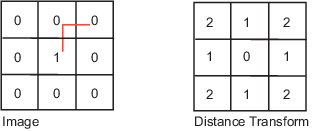
Relationships between pixels(Neighbours and Connectivity)

An image is denoted by f(x,y) and p,q are used to represent individual pixels of the image. Neighbours of a pixel

A pixel p at (x,y) has 4-horizontal/vertical neighbours at (x+1,y), (x-1,y), (x,y+1) and (x,y-1). These are called the 4-neighbours of p : N4(p).

A pixel p at (x,y) has 4 diagonal neighbours at (x+1,y+1), (x+1,y-1), (x-1,y+1) and (x-1,y-1). These are called the diagonal-neighbours of p : ND(p).

The 4-neighbours and the diagonal neighbours of p are called 8-neighbours of p : N8(p).

Adjacency between pixels

Let V be the set of intensity values used to define adjacency.

In a binary image, V ={1} if we are referring to adjacency of pixels with value 1. In a gray-scale image, the idea is the same, but set V typically contains more elements.

For example, in the adjacency of pixels with a range of possible intensity values 0 to 255, set V could be any subset of these 256 values.

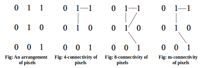
We consider three types of adjacency:

a) 4-adjacency: Two pixels p and q with values from V are 4-adjacent if q is in the set N4(p).

b) 8-adjacency: Two pixels p and q with values from V are 8-adjacent if q is in the set N8(p).

c) m-adjacency(mixed adjacency): Two pixels p and q with values from V are m-adjacent if

q is in N4(p), or
2) q is in ND(p) and the set N4(p)∩N4(q) has no pixels whose values are from V.

Connectivity between pixels

It is an important concept in digital image processing.

It is used for establishing boundaries of objects and components of regions in an image.

Two pixels are said to be connected:

if they are adjacent in some sense(neighbour pixels,4/8/m-adjacency)
if their gray levels satisfy a specified criterion of similarity(equal intensity level)

There are three types of connectivity on the basis of adjacency. They are:

a) 4-connectivity: Two or more pixels are said to be 4-connected if they are 4-adjacent with each others.

b) 8-connectivity: Two or more pixels are said to be 8-connected if they are 8-adjacent with each others.

c) m-connectivity: Two or more pixels are said to be m-connected if they are m-adjacent with each others.

What is adjacency of a pixel?

Adjacency. • Two pixels are connected if they are. neighbors and their gray levels satisfy some specified criterion of similarity. • For example, in a binary image two pixels. are connected if they are 4-neighbors and have same value (0/1).

What are the properties of distance between two pixels?

The Euclidean distance is the straight-line distance between two pixels. The city block distance metric measures the path between the pixels based on a 4-connected neighborhood. Pixels whose edges touch are 1 unit apart; pixels diagonally touching are 2 units apart.

Distance Transform of a Binary Image

The distance transform provides a metric or measure of the separation of points in the image. The bwdist function calculates the distance between each pixel that is set to off (0) and the nearest nonzero pixel for binary images.

The bwdist function supports several distance metrics.

Distance Metrics

Distance Metric	Description	Illustration
Euclidean	The Euclidean distance is the straight-line distance between two pixels.
City Block	The city block distance metric measures the path between the pixels based on a 4-connected neighborhood. Pixels whose edges touch are 1 unit apart; pixels diagonally touching are 2 units apart.
Chessboard	The chessboard distance metric measures the path between the pixels based on an 8-connected neighborhood. Pixels whose edges or corners touch are 1 unit apart.
Quasi-Euclidean	The quasi-Euclidean metric measures the total Euclidean distance along a set of horizontal, vertical, and diagonal line segments.

This example creates a binary image containing two intersecting circular objects.

center1 = -10; 
center2 = -center1; 
dist = sqrt(2*(2*center1)^2); 
radius = dist/2 * 1.4; 
lims = [floor(center1-1.2*radius) ceil(center2+1.2*radius)]; 
[x,y] = meshgrid(lims(1):lims(2)); 
bw1 = sqrt((x-center1).^2 + (y-center1).^2) <= radius; 
bw2 = sqrt((x-center2).^2 + (y-center2).^2) <= radius; 
bw = bw1 | bw2; 
figure
imshow(bw)

To compute the distance transform of the complement of the binary image, use the bwdist function. In the image of the distance transform, note how the centers of the two circular areas are white.